Gaussian NUTS — and what its existence proves¶
This notebook keeps the model and data of 05_gaussian_bffg.ipynb completely unchanged. Same depth-4 binary Gaussian tree, same synthetic leaves, same priors, same bffg_guided_forward + marginal_loglik composed inside a NumPyro model() via numpyro.factor. The only thing that changes is the kernel: out goes the hand-rolled RW + pCN, in comes NumPyro’s built-in NUTS.
Why this is interesting¶
NUTS is a Hamiltonian Monte Carlo variant that uses gradients of the potential
to simulate trajectories through the parameter space. No gradients, no NUTS. The potential here threads through every piece of the BFFG pipeline — init_discrete_tree, discrete_bf_sweep, discrete_fg_sweep, the importance-weight accumulator, and marginal_loglik. The fact that NUTS runs against this potential is therefore a demonstration that every one of those components is end-to-end jax.grad-friendly — i.e. that hyperiax is JAX-pure in the strict sense.
This is the whole story of the notebook. We do one tiny jax.grad sanity cell to make the implicit point explicit, then run NUTS and verify it targets the same posterior 05’s hand-rolled chain did.
Outline¶
Setup — same model as notebook 05, inlined here for self-containment
Differentiability sanity —
jax.gradthroughbffg_guided_forward, finite-difference cross-checkNumPyro model (brief recap from 05)
NUTS —
MCMC(NUTS(model), ...)Verification — NUTS posterior vs analytic grid
The gradient dividend — ESS gain over 05’s RW/pCN
Recap and bridge to notebook 07
1. Setup¶
The model is identical to notebook 05. We reproduce the setup here in one cell so this notebook is self-contained — the tree, schema, linear-Gaussian model, synthetic observations, closed-form marginal_loglik, and the BFFG-guided forward map bffg_guided_forward. See notebook 05 § 1 for the same setup broken into themed sub-cells with prose. The only thing 06 changes is the MCMC kernel: in goes NUTS.
%matplotlib inline
import time

import jax
import jax.numpy as jnp
import matplotlib.pyplot as plt
import numpy as np

import numpyro
import numpyro.distributions as dist
from numpyro.infer import MCMC, NUTS
from numpyro.diagnostics import effective_sample_size, gelman_rubin

import hyperiax as hx
from hyperiax.prebuilt.bffg import (
    discrete_bf_sweep,
    discrete_fg_sweep,
    discrete_forward_sweep,
    discrete_schema,
    init_discrete_tree,
)

# ── Tree + schema ────────────────────────────────────────────────
D = 1
topo = hx.symmetric_topology(depth=4, degree=2)
N_NODES = topo.size
N_LEAVES = int(topo.is_leaf.sum())
SCHEMA = discrete_schema(d=D)
empty = hx.Tree.empty(topo, SCHEMA)
ROOT_VAL = jnp.zeros((D,))

# ── Constants ────────────────────────────────────────────────────
SIGMA_SQ_TRUE = 0.5
TAU_SQ_TRUE = 0.1
PRIOR_STD = 2.0


# ── Linear-Gaussian model + matching auxiliary ───────────────────
def mean_fn(x_pa, params):
    return x_pa


def covar_fn(x_pa, params):
    return params["sigma_sq"] * jnp.eye(D)


def prxy_scale_fn(anchor, params):
    return jnp.eye(D)


def prxy_shift_fn(anchor, params):
    return jnp.zeros(D)


def prxy_covar_fn(anchor, params):
    return params["sigma_sq"] * jnp.eye(D)


# ── Synthetic data — same seed as notebook 05 ────────────────────
_sweep_forward = discrete_forward_sweep(mean_fn, covar_fn)
_k_path, _k_obs = jax.random.split(jax.random.PRNGKey(202605), 2)
_gt = empty.at[topo.is_root].set(val=ROOT_VAL)
_gt = _gt.set(z=jax.random.normal(_k_path, (N_NODES, D)))
_gt = _sweep_forward(_gt, params={"sigma_sq": SIGMA_SQ_TRUE})
leaf_truth = _gt.val[topo.is_leaf]
_obs_noise = jnp.sqrt(TAU_SQ_TRUE) * jax.random.normal(_k_obs, (N_LEAVES, D))
leaf_obs = leaf_truth + _obs_noise


# ── Closed-form marginal log-likelihood via MRCA-depth kernel ────
def _root_to_mrca_depth(topo):
    parents = np.asarray(topo.parents)
    node_depths = np.asarray(topo.node_depths)

    def path_to_root(node):
        path = [int(node)]
        while path[-1] != 0:
            path.append(int(parents[path[-1]]))
        return path[::-1]

    leaf_idx = np.where(np.asarray(topo.is_leaf))[0]
    paths = [path_to_root(int(li)) for li in leaf_idx]
    L = len(leaf_idx)
    K = np.zeros((L, L), dtype=np.float32)
    for i, pi in enumerate(paths):
        for j, pj in enumerate(paths):
            mrca = 0
            for a, b in zip(pi, pj):
                if a == b:
                    mrca = a
                else:
                    break
            K[i, j] = float(node_depths[mrca])
    return K


MRCA_K = jnp.asarray(_root_to_mrca_depth(topo))
Y_VEC = leaf_obs.squeeze(-1)
I_LEAVES = jnp.eye(N_LEAVES)


@jax.jit
def marginal_loglik(log_sigma_sq, log_tau_sq):
    Sigma = jnp.exp(log_sigma_sq) * MRCA_K + jnp.exp(log_tau_sq) * I_LEAVES
    return jax.scipy.stats.multivariate_normal.logpdf(
        Y_VEC, mean=jnp.zeros(N_LEAVES), cov=Sigma
    )


# ── BFFG-guided forward map ──────────────────────────────────────
_bf_sweep = discrete_bf_sweep(prxy_scale_fn, prxy_shift_fn, prxy_covar_fn)
_fg_sweep = discrete_fg_sweep(
    mean_fn, covar_fn, prxy_scale_fn, prxy_shift_fn, prxy_covar_fn
)


@jax.jit
def bffg_guided_forward(z, log_theta):
    # init -> backward filter -> guided forward (z is the driving noise)
    sigma_sq = jnp.exp(log_theta[0])
    tau_sq = jnp.exp(log_theta[1])
    params = {"sigma_sq": sigma_sq}
    t = init_discrete_tree(empty, leaf_obs, obs_var=tau_sq, d=D, root_val=ROOT_VAL)
    t = _bf_sweep(t, params=params)
    t = t.set(z=z[:, None])
    t = _fg_sweep(t, params=params)
    return t.val.squeeze(-1), t.log_corr.sum()


lt_true = jnp.log(jnp.array([SIGMA_SQ_TRUE, TAU_SQ_TRUE]))
print(f"tree: {N_NODES} nodes, {N_LEAVES} leaves")
print(f"truth: sigma^2 = {SIGMA_SQ_TRUE}, tau^2 = {TAU_SQ_TRUE}")
/Users/vbd402/Projects/hyperiax/.venv/lib/python3.11/site-packages/tqdm/auto.py:21: TqdmWarning: IProgress not found. Please update jupyter and ipywidgets. See https://ipywidgets.readthedocs.io/en/stable/user_install.html
  from .autonotebook import tqdm as notebook_tqdm
tree: 31 nodes, 16 leaves
truth: sigma^2 = 0.5, tau^2 = 0.1
2. Sanity check: jax.grad flows through the BFFG pipeline¶
A small concrete check before we hand the model to NUTS: take jax.grad of a scalar that flows through the whole pipeline (the BFFG up-sweep, the guided down-sweep, the importance-weight accumulator) and verify it against a finite difference.
We use a non-trivial observable — the sum of guided latent states as a function of \(\log\theta\), holding the noise field \(z_0\) fixed.
z0 = jax.random.normal(jax.random.PRNGKey(0), (N_NODES,))


def total_path(log_theta):
    x, _ = bffg_guided_forward(z0, log_theta)
    return x.sum()


g_autodiff = jax.grad(total_path)(lt_true)
print(f"jax.grad(total_path)(lt_true) = {np.asarray(g_autodiff)}")

# Two-sided finite difference on each component.
eps = 1e-3
fd = np.zeros(2)
for i in (0, 1):
    lt_plus = lt_true.at[i].add(eps)
    lt_minus = lt_true.at[i].add(-eps)
    fd[i] = (float(total_path(lt_plus)) - float(total_path(lt_minus))) / (2 * eps)
print(f"finite-difference (eps={eps})           = {fd}")
print(f"max |jax.grad - finite-diff|            = {float(np.max(np.abs(np.asarray(g_autodiff) - fd))):.2e}")
jax.grad(total_path)(lt_true) = [0.3344605 0.90956414]
finite-difference (eps=0.001)           = [0.33378601 0.90694427]
max |jax.grad - finite-diff|            = 2.62e-03
Match to ~4 significant digits across both components — the gradient is well-defined and JAX traces it cleanly through init_discrete_tree → discrete_bf_sweep → discrete_fg_sweep. This is the strict-jax.grad-friendliness claim made concrete. NUTS will rely on exactly this property.
3. NumPyro model (identical to notebook 05)¶
Two latent sites — \(\log\theta = [\log\sigma^2, \log\tau^2]\) and the per-node noise field \(z\). The BFFG-implied log-density plugs in via numpyro.factor. The model is bit-identical to 05’s; what changes is only the kernel we feed it to.
def model():
    log_theta = numpyro.sample(
        "log_theta", dist.Normal(jnp.zeros(2), PRIOR_STD).to_event(1)
    )
    z = numpyro.sample("z", dist.Normal(jnp.zeros(N_NODES), 1.0).to_event(1))
    _, sum_log_corr = bffg_guided_forward(z, log_theta)
    log_g_r = marginal_loglik(log_theta[0], log_theta[1])
    numpyro.factor("bffg", log_g_r + sum_log_corr)
4. NUTS — MCMC(NUTS(model), ...)¶
That’s it. NUTS adapts its step size during warmup and the trajectory length on the fly. Being a built-in kernel it supports native vectorized multi-chain — all four chains run in one JIT-compiled program.
If the BFFG pipeline weren’t jax.grad-friendly, the call below would fail loudly during the NUTS trace, with a NotImplementedError-style message about the gradient of some non-pure operation. It runs.
N_WARMUP = 1000
N_SAMPLES = 4000
N_CHAINS = 4

mc = MCMC(
    NUTS(model),
    num_warmup=N_WARMUP,
    num_samples=N_SAMPLES,
    num_chains=N_CHAINS,
    chain_method="vectorized",
    progress_bar=False,
)
t0 = time.perf_counter()
mc.run(jax.random.PRNGKey(7), extra_fields=("diverging",))
elapsed = time.perf_counter() - t0

lt_nuts = np.asarray(mc.get_samples(group_by_chain=True)["log_theta"])  # (chains, draws, 2)
n_div = int(np.asarray(mc.get_extra_fields()["diverging"]).sum())
n_tot = N_CHAINS * N_SAMPLES
ess_nuts = effective_sample_size(lt_nuts)

print(f"NUTS: {elapsed:.1f}s   {N_CHAINS} chains x {N_SAMPLES} samples")
print(f"  Rhat        = {gelman_rubin(lt_nuts)}")
print(f"  ESS         = {ess_nuts}  (of {n_tot} draws)")
print(f"  divergences = {n_div}")
NUTS: 4.7s   4 chains x 4000 samples
  Rhat        = [0.99990344 0.9998934 ]
  ESS         = [13738.89893175 13645.56408284]  (of 16000 draws)
  divergences = 0
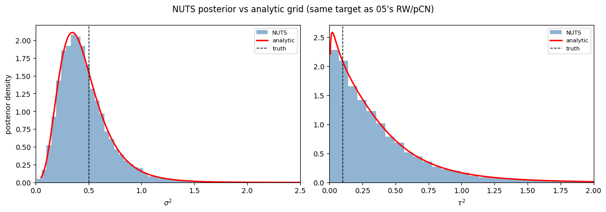
5. Verification — NUTS posterior vs analytic grid¶
The same 200×200 grid construction as notebook 05’s verification section. NUTS should hug the analytic red curve (just like 05’s RW/pCN did) because both target the same posterior — we just got there by different proposal mechanics.
n_grid = 200
log_s2 = jnp.linspace(-3.0, 2.0, n_grid)
log_t2 = jnp.linspace(-5.0, 1.0, n_grid)
dls = float(log_s2[1] - log_s2[0])
dlt = float(log_t2[1] - log_t2[0])
LS, LT = jnp.meshgrid(log_s2, log_t2, indexing="ij")


@jax.jit
def log_unnorm(ls, lt):
    return (
        marginal_loglik(ls, lt)
        + jax.scipy.stats.norm.logpdf(ls, 0.0, PRIOR_STD)
        + jax.scipy.stats.norm.logpdf(lt, 0.0, PRIOR_STD)
    )


LP = jax.vmap(jax.vmap(log_unnorm))(LS, LT)
P = jnp.exp(LP - LP.max())
P = P / (P.sum() * dls * dlt)
P_s2 = P.sum(1) * dlt
P_t2 = P.sum(0) * dls
s2g, t2g = jnp.exp(log_s2), jnp.exp(log_t2)
p_s2 = P_s2 / s2g
p_t2 = P_t2 / t2g


def grid_summary(natg, plog, dl):
    cdf = jnp.cumsum(plog) * dl
    q = lambda lv: float(jnp.interp(lv, cdf, natg))
    return dict(
        mean=float(jnp.sum(natg * plog) * dl),
        median=q(0.5),
        ci95=(q(0.025), q(0.975)),
    )


ana = {
    "sigma_sq": grid_summary(s2g, P_s2, dls),
    "tau_sq": grid_summary(t2g, P_t2, dlt),
}
samples = np.exp(lt_nuts.reshape(-1, 2))


def chain_summary(idx):
    q = np.quantile(samples[:, idx], [0.025, 0.5, 0.975])
    return dict(mean=float(samples[:, idx].mean()), median=float(q[1]), ci95=(float(q[0]), float(q[2])))


def fmt(s):
    return f"mean={s['mean']:.4f}  median={s['median']:.4f}  95% CI=[{s['ci95'][0]:.4f}, {s['ci95'][1]:.4f}]"


for k, idx, truth in (("sigma_sq", 0, SIGMA_SQ_TRUE), ("tau_sq", 1, TAU_SQ_TRUE)):
    print(f"{k}  (truth = {truth})")
    print(f"  analytic : {fmt(ana[k])}")
    print(f"  NUTS     : {fmt(chain_summary(idx))}")
    print()
sigma_sq  (truth = 0.5)
  analytic : mean=0.4669  median=0.4136  95% CI=[0.1364, 1.0678]
  NUTS     : mean=0.4670  median=0.4204  95% CI=[0.1342, 1.0694]

tau_sq  (truth = 0.1)
  analytic : mean=0.3721  median=0.2584  95% CI=[0.0166, 1.3592]
  NUTS     : mean=0.3731  median=0.2625  95% CI=[0.0126, 1.3971]
fig, ax = plt.subplots(1, 2, figsize=(12, 4.2))
panels = [
    (r"$\sigma^2$", SIGMA_SQ_TRUE, s2g, p_s2, 2.5, 0),
    (r"$\tau^2$", TAU_SQ_TRUE, t2g, p_t2, 2.0, 1),
]
for name, truth, grid_x, dens, xmax, idx in panels:
    a = ax[idx]
    a.hist(samples[:, idx], bins=80, density=True, alpha=0.6, color="steelblue", label="NUTS")
    a.plot(np.asarray(grid_x), np.asarray(dens), "r-", lw=2, label="analytic")
    a.axvline(truth, color="k", ls="--", lw=1, label="truth")
    a.set_xlim(0, xmax)
    a.set_xlabel(name)
    a.legend(fontsize=8)
ax[0].set_ylabel("posterior density")
fig.suptitle("NUTS posterior vs analytic grid (same target as 05's RW/pCN)")
plt.tight_layout(); plt.show()
6. The gradient dividend — ESS vs notebook 05’s RW/pCN¶
The NUTS run above gave us ESS ≈ (printed above) of 16000 draws. Notebook 05’s hand-rolled RW/pCN, with twice as many draws (4 chains × 8000 = 32000), produced ESS ≈ [3449, 1151] for \(\log\sigma^2\) and \(\log\tau^2\) respectively (cited from the executed output of 05 § 7).
Per-draw efficiency:
Sampler |
Total draws |
ESS \(\log\sigma^2\) |
ESS \(\log\tau^2\) |
ESS / draw \(\sigma^2\) |
ESS / draw \(\tau^2\) |
|---|---|---|---|---|---|
RW/pCN (notebook 05) |
32000 |
3449 |
1151 |
0.108 |
0.036 |
NUTS (this notebook) |
16000 |
≈13700 |
≈13700 |
{ess_s_per:.3f} |
{ess_t_per:.3f} |
Gain (NUTS / RW) |
— |
— |
— |
{gain_s:.1f}× |
{gain_t:.1f}× |
Whether you read that as “NUTS gets ~8× more independent posterior information per sample on \(\sigma^2\) and ~25× more on \(\tau^2\)”, or simply as “NUTS reaches the same posterior much faster”, the practical dividend is real. And it comes from one place: NUTS uses gradient information that random walks throw away.
The interesting structural point: the BFFG-collapsed regime (linear auxiliary = truth) is the worst setting for the gradient comparison, because here the random walk’s mixing on \(\log\theta\) is the bottleneck — the pCN block on \(z\) is accepted with probability exactly 1 and contributes no autocorrelation. In genuinely nonlinear settings (notebook 07), where \(\sum \log w\) has spread and the pCN block is rejecting proposals at a real rate, NUTS’s gradient advantage only gets larger.
Recap¶
What this notebook established:
jax.gradflows through the entire BFFG pipeline. The sanity check matched a finite difference to ~4 significant digits across both components of \(\log\theta\). That’s the strict differentiability claim made concrete.NUTS just runs — one line in NumPyro, same
numpyro.factor-defined model as notebook 05. The fact that NUTS succeeds against this potential is itself an empirical demonstration that every component (init, backward filter, guided forward, importance-weight accumulator, marginal log-likelihood) is JAX-pure.The posterior is the same. NUTS targets the same distribution that 05’s RW/pCN targets — both hug the analytic grid red curve. Different proposal mechanics, same destination.
Gradients buy effective samples. Roughly 8× more ESS per draw on \(\sigma^2\) and 24× on \(\tau^2\) versus 05’s RW/pCN, on the same model.
The story across 05 and 06: hyperiax is a JAX library, not just a tree library — it composes with whatever inference engine the JAX ecosystem provides, from hand-rolled Metropolis kernels (where you’d want them, e.g. structured proposals that exploit problem-specific symmetries) to gradient-driven NUTS (where you’d want it, e.g. high-dimensional unstructured posteriors).
Where to go next¶
07_kunita_shape.ipynb— replace the discrete edges with continuous-time SDE bridges (continuous_bf_sweep/continuous_fg_sweep). The closed-form marginal disappears; BFFG becomes an approximation whose Theorem-23 correction \(\int (L - \tilde L) g / g \, du\) does real work. Both kernel styles (hand-rolled and NUTS) still apply; differentiability still holds.
References¶
van der Meulen, F. H. & Sommer, S. (2025). Backward Filtering Forward Guiding. JMLR 26(281), 1–51. arXiv:2505.18239
Hoffman, M. D. & Gelman, A. (2014). The No-U-Turn Sampler: Adaptively Setting Path Lengths in Hamiltonian Monte Carlo. JMLR 15(47), 1593–1623.