Quickstart — Hyperiax in five minutes

Hyperiax lets you write tree message-passing algorithms in JAX. The whole user-facing API has four pieces:

Piece	What it is
Topology	The static shape of the tree (who’s whose parent).
Tree	Topology + a typed dict of per-node arrays. Immutable. Registered as a JAX pytree, so it rides through jax.jit / jax.lax.scan / jax.grad cleanly.
@hx.up / @hx.down	Decorators that turn a small Python function into a leaf→root or root→leaf sweep.
Views	Inside a sweep, you read data through node.value, parent.value, children.value.mean(0).

This notebook walks through all four. By the end you will have built a tree, run an up-sweep and a down-sweep, and verified that sweeps compose with jax.jit, jax.lax.scan, and jax.grad.

import jax
import jax.numpy as jnp
import numpy as np
import matplotlib.pyplot as plt

import hyperiax as hx

1. Build a topology

A Topology is a parent-pointer array plus a bunch of precomputed dispatch metadata. The only convention you need to remember:

• Nodes are stored in BFS order: the root is node 0, and parents[i] < i for every other node.

• The root is its own parent (parents[0] == 0).

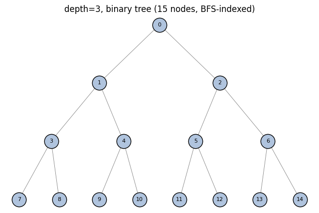
For perfectly symmetric trees there is a convenience constructor. We’ll use a binary tree of height 3 — that’s \(1+2+4+8 = 15\) nodes.

topo = hx.symmetric_topology(depth=3, degree=2)

print(topo)
print(f"  size:         {topo.size}")
print(f"  depth:        {topo.depth}")
print(f"  num leaves:   {int(topo.is_leaf.sum())}")
print(f"  equal_degree: {topo.equal_degree}")
print(f"  parents:      {topo.parents.tolist()}")

Topology(size=15, depth=3, equal_degree=True, max_degree=2)
  size:         15
  depth:        3
  num leaves:   8
  equal_degree: True
  parents:      [0, 0, 0, 1, 1, 2, 2, 3, 3, 4, 4, 5, 5, 6, 6]

A tiny matplotlib helper so we can see what’s going on. Reuse this cell whenever you want to draw a tree.

topo.parents, topo.level_starts, topo.is_leaf, … are all numpy arrays — the topology lives in numpy-land so it can ride through jax.jit as static auxiliary data.

def plot_tree(topo, values=None, ax=None, title=None, cmap='viridis', vmin=None, vmax=None):
    """Top-down layered layout. Pass `values` (shape (N,)) to color nodes."""
    if ax is None:
        _, ax = plt.subplots(figsize=(8, 5))
    pos = np.zeros((topo.size, 2))
    for d in range(topo.depth + 1):
        lo, hi = int(topo.level_starts[d]), int(topo.level_starts[d + 1])
        n = hi - lo
        if n == 1:
            pos[lo:hi, 0] = 0.5
        else:
            pos[lo:hi, 0] = np.linspace(0, 1, n + 2)[1:-1]
        pos[lo:hi, 1] = -d
    for i in range(1, topo.size):
        p = int(topo.parents[i])
        ax.plot([pos[p, 0], pos[i, 0]], [pos[p, 1], pos[i, 1]],
                'k-', lw=0.6, alpha=0.5, zorder=1)
    if values is None:
        ax.scatter(pos[:, 0], pos[:, 1], s=420, c='lightsteelblue',
                   edgecolor='k', zorder=3)
        for i in range(topo.size):
            ax.text(pos[i, 0], pos[i, 1], str(i), ha='center', va='center', fontsize=8)
    else:
        sc = ax.scatter(pos[:, 0], pos[:, 1], s=420, c=np.asarray(values),
                        edgecolor='k', cmap=cmap, vmin=vmin, vmax=vmax, zorder=3)
        plt.colorbar(sc, ax=ax, label='value', shrink=0.8)
    if title:
        ax.set_title(title)
    ax.set_axis_off()
    return ax

plot_tree(topo, title=f"depth={topo.depth}, binary tree ({topo.size} nodes, BFS-indexed)")
plt.show()

2. Declare a schema, allocate a Tree

A Tree is Topology + a dict[str, jax.Array] whose keys are fixed by a schema. You declare what fields exist up front:

Tree.empty(topo, {'value': trailing_shape, ...})

Each field has a (trailing_shape, dtype) spec — () for a scalar field, (2,) for a 2-vector field, (n, n) for a matrix field, and so on. The leading axis is always the number of nodes; the schema only declares the trailing part.

Why declare it up front? The schema is part of the pytree’s static aux data. Adding fields later via tree.update(...) changes the pytree structure and invalidates jit caches keyed on the old shape. Inside a sweep pipeline you almost always know all your fields at construction time.

tree = hx.Tree.empty(topo, {'value': ()})
print(tree)
print("Initial values (zeros for every node):")
print(tree.value)
print("Allocate shape (leading dimension is the number of nodes):")
print(tree.value.shape)

Tree(size=15, fields={value: ()})
Initial values (zeros for every node):
[0. 0. 0. 0. 0. 0. 0. 0. 0. 0. 0. 0. 0. 0. 0.]
Allocate shape (leading dimension is the number of nodes):
(15,)

3. Seed the leaves

Trees are immutable. Every “mutator” — set, at[...].set/add/..., update, drop — returns a new Tree. This is what lets us put the whole computation inside jax.jit.

tree.at[mask_or_indices].set(field=values) is the JAX-style scatter — same shape as arr.at[mask].set(values), but takes the field name(s) as keyword arguments. The at[...] indexer also exposes add, multiply, min, max, and get.

num_leaves = int(topo.is_leaf.sum())                # 8
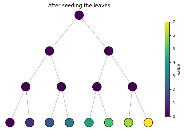
leaf_obs = jnp.arange(num_leaves, dtype=jnp.float32)

tree = tree.at[topo.is_leaf].set(value=leaf_obs)
print("Leaves carry 0..7; inner nodes are still zero:")
print(tree.value)

plot_tree(topo, tree.value, title="After seeding the leaves")
plt.show()

Leaves carry 0..7; inner nodes are still zero:
[0. 0. 0. 0. 0. 0. 0. 0. 1. 2. 3. 4. 5. 6. 7.]

Aside: the full tree.at[...] interface

tree.at[indices] mirrors jax.numpy.ndarray.at[i] but lifts it to a multi-field container. The indexer exposes six operations:

op	what it does	returns
.set(field=v, ...)	scatter-assign	new Tree
.add(field=v, ...)	scatter-add	new Tree
.multiply(field=v, ...)	scatter-multiply	new Tree
.min(field=v, ...)	elementwise min at indices	new Tree
.max(field=v, ...)	elementwise max at indices	new Tree
.get()	read every field at indices	dict[str, jax.Array]

All five write ops accept any number of fields as keyword arguments (one scatter pass per field, all sharing the same indices). All of them are pure: the original tree is unchanged.

# Build a throwaway two-field tree to show every op on the same indices.
demo = (
    hx.Tree.empty(topo, {'value': (), 'count': ()})
      .at[topo.is_leaf].set(value=leaf_obs, count=jnp.ones(num_leaves))
)
print("seed (leaves only):           ", np.asarray(demo.value))

# .add — bump every leaf by 10
bumped = demo.at[topo.is_leaf].add(value=jnp.full(num_leaves, 10.0))
print(".add(+10) at leaves:          ", np.asarray(bumped.value))

# .multiply — scale every leaf's count by 7 (inner-node counts start at 0,
# multiplying them by 7 would be invisible)
scaled = demo.at[topo.is_leaf].multiply(count=jnp.full(num_leaves, 7.0))
print(".multiply(*7) at leaves.count:", np.asarray(scaled['count']))

# .min / .max — clamp the leaves into [2, 5]
clipped = (
    demo.at[topo.is_leaf].max(value=jnp.full(num_leaves, 2.0))
        .at[topo.is_leaf].min(value=jnp.full(num_leaves, 5.0))
)
print(".max(>=2) then .min(<=5):     ", np.asarray(clipped.value))

# .get — read all fields at a set of indices, returns a plain dict
snapshot = demo.at[topo.is_leaf].get()
print(".get() at leaves keys/shape:  ", {k: v.shape for k, v in snapshot.items()})

# Original is untouched (pure functional updates)
print("original demo.value is intact:", np.asarray(demo.value))

seed (leaves only):            [0. 0. 0. 0. 0. 0. 0. 0. 1. 2. 3. 4. 5. 6. 7.]
.add(+10) at leaves:           [ 0.  0.  0.  0.  0.  0.  0. 10. 11. 12. 13. 14. 15. 16. 17.]
.multiply(*7) at leaves.count: [0. 0. 0. 0. 0. 0. 0. 7. 7. 7. 7. 7. 7. 7. 7.]
.max(>=2) then .min(<=5):      [0. 0. 0. 0. 0. 0. 0. 2. 2. 2. 3. 4. 5. 5. 5.]
.get() at leaves keys/shape:   {'count': (8,), 'value': (8,)}
original demo.value is intact: [0. 0. 0. 0. 0. 0. 0. 0. 1. 2. 3. 4. 5. 6. 7.]

4. An up-sweep: propagate information leaf → root

An up-sweep visits every level from the leaves toward the root. At each non-leaf node, your function receives:

• node — the node’s own fields. Each attribute has shape (*trailing,) (one node at a time, courtesy of jax.vmap inside the dispatcher).

• children — the children of this node. For an equal-degree tree, children.value is a real JAX array of shape (k, *trailing) — slice it, multiply it, sum it like any other array. For unequal-degree trees, the same expression works through a ChildrenAxis proxy that dispatches reductions to jax.ops.segment_*.

• params — whatever you pass via sweep(tree, params=...) (a dict, an array, anything pytree-shaped).

Your function returns a dict whose keys exactly match the writes= argument. Each value must have shape (*trailing,) — one record per node, no need to keep a per-parent batch axis.

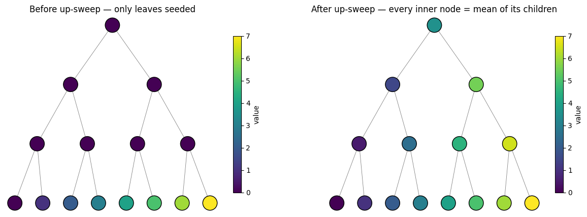
We’ll compute the simplest message possible: each non-leaf node = mean of its children.

@hx.up(reads_children=('value',), writes=('value',))
def average_children(node, children, params):
    return {'value': children.value.mean(0)}

tree_after_up = average_children(tree)

print("Root value after up-sweep: ", float(tree_after_up.value[0]))
print("Mean of the leaves:        ", float(leaf_obs.mean()))
print("All node values:\n", np.asarray(tree_after_up.value))

Root value after up-sweep:  3.5
Mean of the leaves:         3.5
All node values:
 [3.5 1.5 5.5 0.5 2.5 4.5 6.5 0.  1.  2.  3.  4.  5.  6.  7. ]

fig, axes = plt.subplots(1, 2, figsize=(15, 5))
vmin, vmax = 0.0, float(num_leaves - 1)
plot_tree(topo, tree.value, ax=axes[0],
          title="Before up-sweep — only leaves seeded", vmin=vmin, vmax=vmax)
plot_tree(topo, tree_after_up.value, ax=axes[1],
          title="After up-sweep — every inner node = mean of its children",
          vmin=vmin, vmax=vmax)
plt.show()

Two things to notice:

1. tree itself is unchanged. average_children returned a brand-new Tree. This is what lets jax.jit see the call as a pure function.

2. We only declared reads_children=('value',). We did not declare reads= on the node itself, because the function doesn’t read it. If you forget to declare a field that you actually read, you’ll get a clear AttributeError pointing at the missing entry — the dispatcher only hands you the fields you asked for.

5. A down-sweep: propagate information root → leaf

The mirror image. Your function receives (node, parent, params); for each non-root node, parent.value is a (*trailing,) view of that node’s parent (already updated by the sweep when it visits the level above).

The root is not visited (it has no parent), so you must seed it manually before calling the sweep.

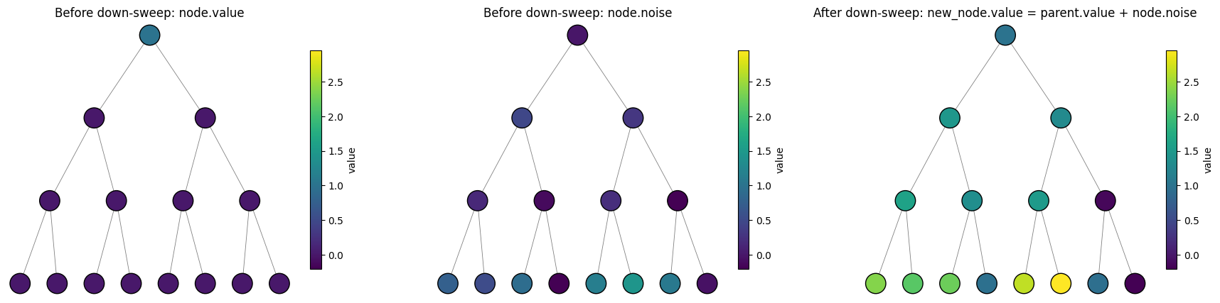
Here we use two fields: a noise we’ll set per node, and a value whose root we’ll seed. The sweep then propagates value = parent.value + noise down the tree.

tree_down = hx.Tree.empty(topo, {'value': (), 'noise': ()})

tree_down = tree_down.at[topo.is_root].set(value=jnp.array([1.0]))
tree_down = tree_down.set(noise=jax.random.normal(jax.random.PRNGKey(42), (topo.size,), dtype=jnp.float32))

@hx.down(reads=('noise',), reads_parent=('value',), writes=('value',))
def propagate(node, parent, params):
    return {'value': parent.value + node.noise}

tree_down_done = propagate(tree_down)

print("Root (kept):       ", float(tree_down_done.value[0]))
print("Children of root:  ", np.asarray(tree_down_done.value[1:3]))
print("All values:\n", np.asarray(tree_down_done.value))

fig, axes = plt.subplots(1, 3, figsize=(22, 5))
vmin, vmax = float(tree_down_done.value.min()), float(tree_down_done.value.max())
plot_tree(topo, tree_down.value, ax=axes[0],
          title="Before down-sweep: node.value", vmin=vmin, vmax=vmax)
plot_tree(topo, tree_down.noise, ax=axes[1],
          title="Before down-sweep: node.noise", vmin=vmin, vmax=vmax)
plot_tree(topo, tree_down_done.value, ax=axes[2],
          title="After down-sweep: new_node.value = parent.value + node.noise", vmin=vmin, vmax=vmax)
plt.show()

Root (kept):        1.0
Children of root:   [1.4671319 1.2957029]
All values:
 [ 1.          1.4671319   1.2957029   1.6206777   1.343099    1.512626
 -0.14517605  2.3765376   2.1420875   2.2532694   0.9586024   2.6524494
  2.9584122   0.9357306  -0.20146927]

6. Sweeps compose with jit, scan, grad

This is the headline feature of v3. A Tree is a JAX pytree (data values are leaves; topology + schema are static aux data), and every sweep is a pure Tree → Tree. That means all of JAX’s transformations work directly.

6a. jax.jit

Wrap the sweep in jax.jit. The first call compiles; subsequent calls on trees with the same structure hit the cache.

print("Unjitted call:")
%timeit _ = average_children(tree)  # JIT-compile the function, but not the call.

jitted_average_children = jax.jit(average_children)
_ = jitted_average_children(tree)  # first-time JIT-compile the function

print("JIT-compiled call:")
# Second call hits the cache — no recompile.
%timeit _ = jitted_average_children(tree)

Unjitted call:
7.55 μs ± 96.4 ns per loop (mean ± std. dev. of 7 runs, 100,000 loops each)
JIT-compiled call:
5.43 μs ± 23.9 ns per loop (mean ± std. dev. of 7 runs, 100,000 loops each)

6b. jax.lax.scan

Iterate the same sweep N times in one compiled XLA loop. The pitch: the body traces once, no per-iteration Python overhead, the whole loop becomes a single device launch.

Two things worth knowing:

1. Always wrap jax.lax.scan in jax.jit. Called eagerly (with no outer jit), lax.scan re-traces its body on every invocation — the inner def body(...) is a fresh Python closure each call, and that per-call tracing dominates everything else, often making scan look slower than a plain Python for-loop. Inside an outer jit, the scan op fuses into the surrounding XLA program and per-call overhead disappears.

2. A Python for-loop can be jit’d, but it unrolls at trace time — the compiled program ends up containing N copies of the body. Trace and compile time both scale linearly with N; at large N this becomes impractical (think tens of seconds, then minutes), while scan compiles in roughly constant time regardless of N. This is why scan is the standard idiom for any non-trivial number of iterations.

Two benchmarks below: (a) runtime — plain Python for-loop vs scan-in-jit (both block_until_ready’d, since JAX dispatches kernels asynchronously and a naive %timeit over a for-loop would otherwise only measure dispatch latency); (b) compile time — scan-in-jit vs the same Python loop wrapped in jit (which forces unrolling). We use N = 1000 and the unrolled side easily takes minutes.

import time

# Bigger tree so the per-iter body work isn't completely drowned out.
big_topo = hx.symmetric_topology(depth=10, degree=2)              # 2047 nodes
big_tree = (
    hx.Tree.empty(big_topo, {'value': ()})
      .at[big_topo.is_leaf].set(value=jnp.ones(int(big_topo.is_leaf.sum())))
)
print(f"benchmark tree: {big_topo.size} nodes, depth={big_topo.depth}")

N = 1000

def for_loop(tree):                              # Python loop of jit'd calls
    for _ in range(N):
        tree = average_children(tree)
    return tree

@jax.jit
def scan_loop(tree):                             # one trace, one XLA scan op
    def body(t, _):
        return average_children(t), None
    final, _ = jax.lax.scan(body, tree, xs=None, length=N)
    return final

@jax.jit
def unrolled_loop(tree):                         # Python loop, body inlined N×
    for _ in range(N):
        tree = average_children(tree)
    return tree

# --- (a) runtime, post-compile, both block_until_ready ---
_ = jax.block_until_ready(scan_loop(big_tree).value)            # warm scan

print("\n=== runtime (post-compile) ===")
print("Python for-loop of jit'd calls:")
%timeit jax.block_until_ready(for_loop(big_tree).value)
print("scan inside jit:")
%timeit jax.block_until_ready(scan_loop(big_tree).value)

# --- (b) compile time: scan vs unrolled jit ---
def measure_compile(fn, arg):
    """Trace + lower + XLA-compile a fresh jit wrapper, return seconds."""
    t0 = time.perf_counter()
    _ = jax.jit(fn).lower(arg).compile()
    return time.perf_counter() - t0

def _scan_fresh(t):
    def body(s, _): return average_children(s), None
    out, _ = jax.lax.scan(body, t, xs=None, length=N)
    return out

def _unrolled_fresh(t):
    for _ in range(N):
        t = average_children(t)
    return t

print(f"\n=== compile time (N = {N}) ===")
print(f"  scan inside jit ({N} iters, body traced 1×):   {measure_compile(_scan_fresh, big_tree):7.2f} s")
print(f"  unrolled for-loop in jit (body inlined {N}×):  {measure_compile(_unrolled_fresh, big_tree):7.2f} s")

benchmark tree: 2047 nodes, depth=10

=== runtime (post-compile) ===
Python for-loop of jit'd calls:
10.8 ms ± 362 μs per loop (mean ± std. dev. of 7 runs, 100 loops each)
scan inside jit:
1.61 ms ± 13.5 μs per loop (mean ± std. dev. of 7 runs, 1,000 loops each)

=== compile time (N = 1000) ===
  scan inside jit (1000 iters, body traced 1×):      0.06 s

E0520 16:39:43.222145  944354 slow_operation_alarm.cc:73] 
********************************
[Compiling module jit__unrolled_fresh for CPU] Very slow compile? If you want to file a bug, run with envvar XLA_FLAGS=--xla_dump_to=/tmp/foo and attach the results.
********************************
E0520 16:43:46.854518  944352 slow_operation_alarm.cc:140] The operation took 6m3.638498s

********************************
[Compiling module jit__unrolled_fresh for CPU] Very slow compile? If you want to file a bug, run with envvar XLA_FLAGS=--xla_dump_to=/tmp/foo and attach the results.
********************************

  unrolled for-loop in jit (body inlined 1000×):   373.14 s

6c. jax.grad

Differentiate end-to-end. Here we treat the leaf observations as the inputs and the root value as the output. With a mean sweep on a height-3 binary tree, each leaf contributes \(1/8\) to the root.

def root_from_leaves(leaf_vals):
    t = hx.Tree.empty(topo, {'value': ()})
    t = t.at[topo.is_leaf].set(value=leaf_vals)
    return average_children(t).value[0]

grads = jax.grad(root_from_leaves)(leaf_obs)
print("d(root) / d(leaves) =", np.asarray(grads))
print("expected: 1/8 for each of the 8 leaves =", 1.0 / num_leaves)

d(root) / d(leaves) = [0.125 0.125 0.125 0.125 0.125 0.125 0.125 0.125]
expected: 1/8 for each of the 8 leaves = 0.125

Recap & next steps

You’ve now seen the entire core API:

• hx.symmetric_topology(height, degree) (and hx.from_parents(parents) for arbitrary topologies)

• hx.Tree.empty(topo, schema), tree.set(...), tree.at[mask].set(...)

• tree.value for field access (or tree['value'] when the field name is a dynamic string or collides with a reserved name like size)

• @hx.up(reads_children=, writes=) with (node, children, params) -> dict

• @hx.down(reads_parent=, writes=) with (node, parent, params) -> dict

• node.value, children.value.mean(0), parent.value inside a sweep

• Sweeps compose with jax.jit, jax.lax.scan, jax.grad directly

Where to go next:

• 02_writing_sweeps.ipynb — go deeper: equal vs unequal degree trees, the reads / reads_children / reads_parent / writes declaration model, custom reductions on the children axis, common patterns (subtree sizes, max depth, weighted means, belief propagation).

• 03_phylo_mean.ipynb — read a real Newick tree, run the phylo_mean prebuilt on it.

• 04_phylo_bayesian.ipynb — upgrade the point estimate to a full Bayesian posterior over ancestral states.